Throttle Body Effective Area: Why Your Table Isn't Linear

Open any modern standalone ECU that runs a throttle-based air model and you’ll find a table mapping throttle position to flow area. Open a dozen real calibrations and a good number of those tables will be a straight line from zero to full scale.

A straight line is the one shape the table physically cannot be.

This isn’t a precision quibble. In the operating band where the engine spends most of its life, meaning idle, overrun, light cruise and the first few percent of tip-in, a linear table over-states flow area by a factor of two to four. Every downstream calculation inherits that error: fuel mass, torque estimation, pedal mapping, and on a drive-by-wire car, the inverse map the controller uses to decide where to put the plate.

This article covers the geometry of why, the compressible flow equations that turn area into mass, what a throttle mass flow (TMF) model does with the result, and a repeatable method for building a table that’s correct rather than convenient.

Part 1: The geometry

The projection

A butterfly valve is a disc on a shaft in a cylindrical bore. Air gets past it through whatever cross-section the disc doesn’t block, viewed along the bore axis.

Set up coordinates: the bore axis is z, the shaft runs along x, and the plate rotates about the shaft. Call the plate’s angle from the bore-normal plane α, and the angle it sits at when hard against the closed stop α₀.

For the plate to seal in a cylindrical bore at angle α₀, it can’t be a circle. The intersection of a cylinder of radius R with a plane tilted at α₀ is an ellipse with semi-axes R and R/cos α₀. So the plate is elliptical, with the long axis running across the shaft.

Project that plate onto the plane normal to the flow at an arbitrary angle α, and you get an ellipse with semi-axes:

R along the shaft
R · cos α / cos α₀ across it

Which gives the blocked area directly:

A_blocked = πR² · (cos α / cos α₀)

And therefore:

A_open = πR² · (1 − cos α / cos α₀)

Two sanity checks. At α = α₀ the cosine ratio is 1 and open area is zero, because the plate fills the bore. At α = 90° the ratio is zero, open area equals bore area, and the plate is edge-on. Both correct.

Why it can’t be linear

Differentiate the open area with respect to α:

dA/dα = πR² · sin α / cos α₀

Near the closed position, sin α is small. The area barely moves. Expand the cosine for small openings and you get area growing with the square of the angle, not the first power:

1 − cos α ≈ α² / 2

A quadratic. That’s the whole argument. The throttle plate has to swing through a meaningful angle before it uncovers meaningful area, because at small angles you’re only exposing the thin crescent at the edge of a tilted ellipse.

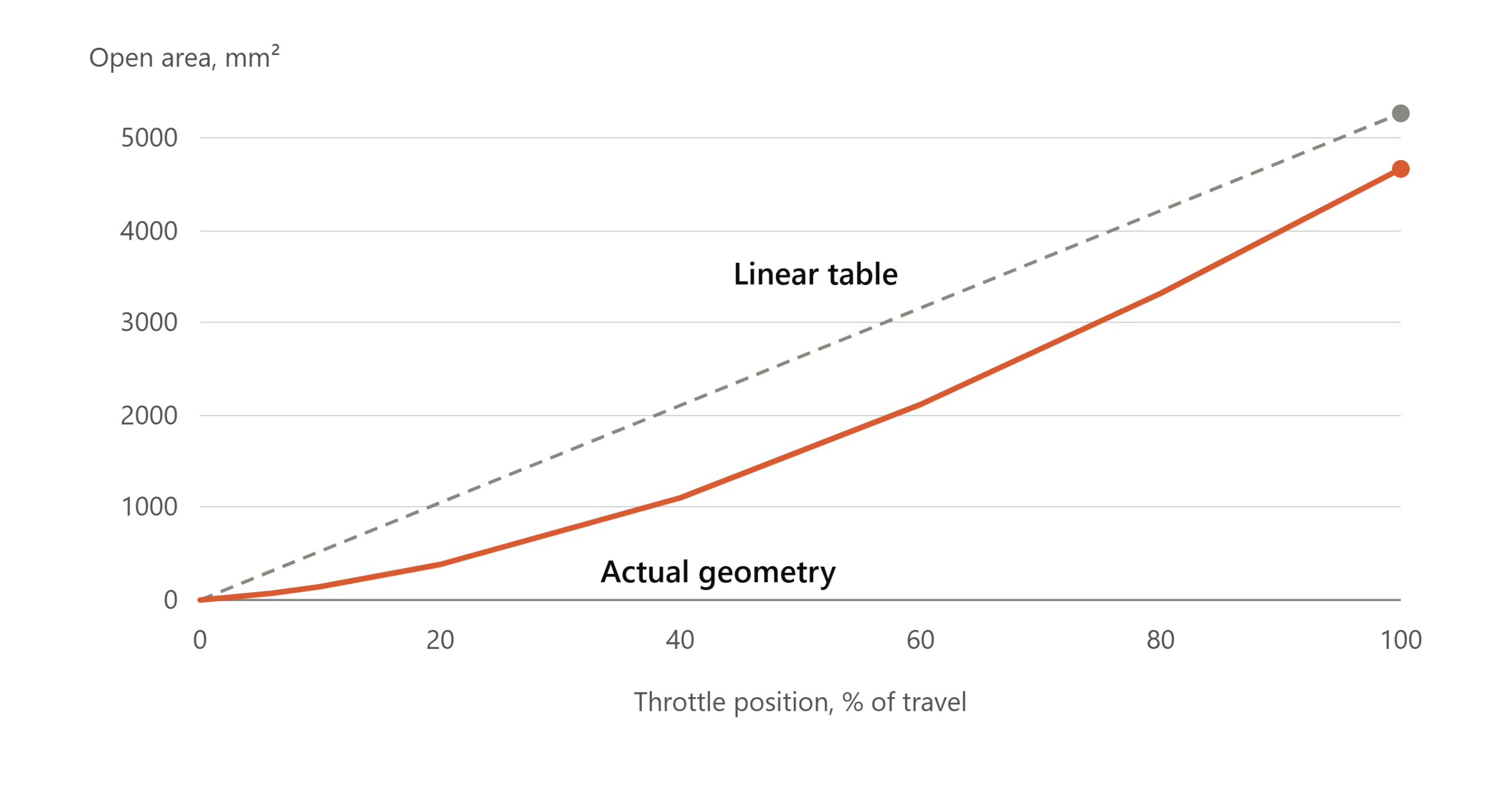
Put numbers on it. Take an 82 mm bore, a closed angle of 9°, an open stop at 83°, and a throttle position axis that runs 0 to 100% of mechanical travel:

TPS %	Plate angle	Open area (mm²)	% of bore	Linear table says	Error
2	10.5°	20	0.4%	106	5.3×
6	13.4°	81	1.5%	317	3.9×
10	16.4°	151	2.9%	528	3.5×
20	23.8°	389	7.4%	1056	2.7×
40	38.6°	1102	20.9%	2112	1.9×
60	53.4°	2124	40.2%	3169	1.5×
80	68.2°	3320	62.9%	4225	1.3×
100	83.0°	4677	88.6%	5281	1.1×

(Bore area 5281 mm². Shaft blockage included, see below. Linear column assumes full scale = bore area.)

The error is worst exactly where it hurts most. A big throttle on a big engine cruises at single-digit TPS. That’s the region where a linear table is out by a factor of four.

The shaft

The shaft blocks area too, but not in the way most people assume. Its projected area is roughly shaft diameter × bore diameter, so call it 8 mm × 82 mm ≈ 656 mm², over 12% of the bore.

But at small openings the shaft is hidden behind the plate’s projection. The plate’s projected ellipse is nearly as wide as the bore, and the shaft sits along its centreline. Shaft blockage only becomes real once the plate has swung far enough that its projection narrows past the shaft width, which on typical geometry is somewhere past 60 to 70°.

So the shaft is irrelevant at idle and dominant at wide-open throttle. If you’ve ever wondered why a throttle body flows meaningfully less than its nominal bore area suggests at WOT, that’s most of the answer.

What the closed-form misses

The clean equation above is a thin-plate, sharp-edged idealisation. Real hardware has:

Plate thickness. A 2 mm plate at 15° presents a real edge to the flow, not a mathematical line.
A seal taper or step in the bore at the closed position, common on OEM bodies to control leakage and stop the plate binding.
A relieved or chamfered plate edge, which changes the effective flow path at small angles specifically.
Screw heads on the plate face where it’s fastened to the shaft.
Non-concentricity between the plate’s rotation axis and the bore centreline on some designs.

None of these are worth modelling analytically. Integrate the geometry numerically and stop pretending you have a closed form. The code is fifteen lines and it handles the shaft correctly for free.

import numpy as np

def open_area(alpha_deg, alpha0_deg, bore_d, shaft_d, n=2000):
    """
    Geometric open area of a butterfly valve, by numerical integration.

    alpha_deg  : plate angle from the bore-normal plane (deg); ~90 = fully open
    alpha0_deg : plate angle at the closed stop (deg)
    bore_d     : bore diameter (mm)
    shaft_d    : shaft diameter (mm)

    Returns (area_mm2, fraction_of_bore_area)
    """
    R  = bore_d / 2.0
    a  = np.deg2rad(alpha_deg)
    a0 = np.deg2rad(alpha0_deg)

    # projected plate ellipse: semi-axis R along shaft, R*cos(a)/cos(a0) across
    sx = R
    sy = max(R * np.cos(a) / np.cos(a0), 1e-12)

    g = np.linspace(-R, R, n)
    X, Y = np.meshgrid(g, g)

    in_bore  = (X**2 + Y**2) <= R**2
    in_plate = ((X / sx)**2 + (Y / sy)**2) <= 1.0
    in_shaft = np.abs(Y) <= shaft_d / 2.0

    cell = (2 * R / (n - 1))**2
    area = np.count_nonzero(in_bore & ~in_plate & ~in_shaft) * cell
    return area, area / (np.pi * R**2)


def servo_to_angle(tps_pct, alpha0_deg, alpha_max_deg):
    """Linear travel-to-angle map. Verify this on your own hardware."""
    return alpha0_deg + (tps_pct / 100.0) * (alpha_max_deg - alpha0_deg)


for tps in [0, 1, 2, 3, 5, 8, 12, 20, 30, 45, 60, 80, 100]:
    ang = servo_to_angle(tps, 9.0, 83.0)
    a, f = open_area(ang, 9.0, 82.0, 8.0)
    print(f"{tps:5.1f}%  {ang:5.1f}°  {a:8.1f} mm²  {f*100:5.2f}%")

Servo position is not plate angle

The table’s axis is usually servo or throttle position in percent. That is a percentage of mechanical travel, mapped through the sensor calibration. It is not plate angle, and it is not flow area.

Two things break here routinely:

The zero point. TPS 0% is wherever the sensor was zeroed, which is typically the closed stop. But the closed stop is often set slightly below the sealing angle so the plate loads against it, or slightly above so it doesn’t jam. If your assumed α₀ is a degree out, your area predictions at low TPS are out by a large multiple, because you’re on the steepest part of a quadratic.

The full-scale point. Plates rarely reach 90°. Mechanical stops usually land somewhere between 80° and 86°, and the linkage may not be perfectly linear across the range. On a DBW body with a direct gear train it’s close enough to linear to be usable. Verify rather than assume.

Measure both. Command the throttle to a known position, remove the intake pipe, and measure the plate angle directly. A digital angle gauge against the plate face is good to a few tenths of a degree, which is plenty. Do it at 0%, 100%, and three or four points in between to confirm linearity. This is twenty minutes of work that determines whether everything downstream is right or wrong.

The scaling trap

If a table has been carried over from a different throttle body, check what it was scaled by.

Area scales with the square of diameter. Going from 68 mm to 82 mm:

Diameter ratio: 82 / 68 = 1.206
Area ratio: 82² / 68² = 1.454

Scale by diameter instead of area and every entry is 17% low. That’s the obvious error.

The subtler one: even a correctly area-scaled table has the wrong shape. Closed angle, open stop angle, and shaft-to-bore ratio all differ between bodies, and none of them scale with diameter. The same shaft in a smaller bore blocks a larger fraction of it. A table lifted from another throttle body and multiplied by a constant is wrong in a way no single multiplier can fix.

Part 2: From area to mass flow

Geometric area isn’t flow area. Two corrections stand between them.

Discharge coefficient

Real flow through an orifice separates at the edge and forms a vena contracta narrower than the geometric opening. The ratio of actual to ideal flow is the discharge coefficient, Cd.

For a butterfly valve, Cd is a function of plate angle, and to a lesser extent of Reynolds number and pressure ratio. Typical values sit somewhere in the 0.6 to 0.8 range across most of the travel, though published data varies considerably with plate profile and bore geometry. The behaviour at very small openings, where the flow is a thin slot jet past a tilted edge, is the least consistent across sources.

If your ECU exposes a separate Cd or flow-correction table against angle, keep the geometric table geometric and put the empirical correction in the Cd table. Two tables, two jobs, and you can reason about each independently. If it only exposes one “effective area” table, you’re folding Cd into it, which works, but means the table is no longer verifiable against geometry, and you lose the ability to sanity-check it with a ruler and a protractor.

The compressible flow equation

Air through a restriction is compressible. The standard isentropic nozzle relation:

ṁ = Cd · A · (P_up / √(R_s · T_up)) · Ψ(PR)

where PR = P_down / P_up, R_s = 287 J/kg·K, and Ψ depends on whether the flow is choked.

Critical pressure ratio for air (γ = 1.4):

PR_crit = (2 / (γ+1))^(γ/(γ-1)) = 0.528

Subsonic (PR > 0.528):

Ψ = √( (2γ/(γ-1)) · ( PR^(2/γ) − PR^((γ+1)/γ) ) )

Choked (PR ≤ 0.528):

Ψ = √γ · (2/(γ+1))^((γ+1)/(2(γ-1))) = 0.6847

Both expressions agree at PR = 0.528, as they must.

The consequence nobody expects: your throttle is choked at idle

Idle manifold pressure on a healthy engine might be 35 kPa absolute, against roughly 101 kPa ambient upstream. That’s a pressure ratio of 0.35, well below critical.

The throttle is sonic. Flow is at the speed of sound in the gap between plate and bore.

That has a specific and useful consequence: when choked, mass flow depends only on Cd, area, upstream pressure and upstream temperature. Manifold pressure has no influence whatsoever. Ψ is pinned at 0.6847 and stays there.

Which means at idle, the model reduces to:

ṁ = Cd · A · P_ambient / √(R_s · T_up) · 0.6847

Every percent of error in your area table becomes a percent of error in calculated air mass, with nothing to absorb it. There is no MAP feedback, no VE term, no second path. Area is the model.

Work out where choking ends: PR = 0.528 against 101 kPa ambient means MAP = 53 kPa. Anything below that is choked, which covers idle, overrun, and most light-load cruise on a large-displacement engine. A big proportion of normal driving sits in the region where the area table is the sole determinant of calculated airflow.

This is the single strongest reason to get the table right, and the reason area errors show up as idle and cruise fuelling problems specifically.

The boosted case, and why pre-throttle pressure matters

Now put the throttle under boost. Upstream is charge pipe pressure, say 200 kPa absolute; downstream is plenum, say 190 kPa. PR = 0.95. Deeply subsonic, and this is where Ψ gets vicious.

Run the numbers:

PR	Ψ
0.96	0.276
0.95	0.306
0.94	0.335
0.93	0.361

A 1% change in pressure ratio produces roughly a 9% change in mass flow. The function is nearly vertical up here.

Which brings us to the thing that decides whether a throttle model can work in boost at all: you must know the pressure upstream of the throttle plate.

Without a pre-throttle sensor, the ECU has to infer it, usually from a modelled pressure drop across the intercooler and pipework, or from a boost target, or by assuming it equals MAP plus some offset. All of those are estimates, and the sensitivity above means a 2 kPa estimation error at part throttle in boost produces a double-digit percentage error in calculated air mass.

Fit the sensor. On a naturally aspirated engine you can argue that ambient is close enough. On a boosted engine running a throttle-based air model, a pre-throttle pressure sensor is not an optional refinement. It’s the difference between a model and a guess.

Note also that the sign of the problem inverts across the throttle range. At small openings the pressure ratio is low, the flow is choked or near-choked, and the model is insensitive to downstream pressure but exquisitely sensitive to area. At large openings in boost the pressure ratio approaches unity, area error matters less, and pressure error dominates. Different regions of the same table fail for different reasons.

Part 3: What the ECU does with it

The throttle mass flow model

A throttle mass flow model, TMF in Emtron’s vocabulary, with equivalents under different names across most modern standalone platforms, computes cylinder air mass from the throttle rather than from the manifold.

Broadly:

Throttle position → plate angle (via the servo map)
Plate angle → geometric area (via the area table)
Area × Cd → effective area
Effective area + upstream pressure + upstream temperature + pressure ratio → mass flow through the throttle
Mass flow → cylinder filling → fuel

Contrast that with speed density, which computes cylinder air mass from manifold pressure, air temperature, engine speed and a volumetric efficiency table.

The two models fail in opposite ways, which is precisely why good ECUs run both:

Speed density is accurate in steady state because MAP is a direct measurement of what’s actually in the manifold. It’s late in transients, because the manifold takes time to fill and the sensor reports the result rather than the intent. Stab the throttle and the MAP sensor tells you what happened a few tens of milliseconds ago.

Throttle mass flow is immediate, because the plate moves before the manifold responds, so the model sees the demand as it happens. But it’s an inference stacked on a chain of assumptions: area table, Cd, servo map, upstream pressure. Every one of those is a place to be wrong.

So the ECU blends them: TMF-weighted during transients where response matters, SD-weighted in steady state where accuracy matters, with a handover region between.

Diagnosing the handover

The handover is where calibration errors become visible, and it’s diagnostically valuable for exactly that reason. If your two models disagree, the blend region will show a fuelling discontinuity that tracks the blend weighting rather than any physical parameter.

Log fuel trim, or measured lambda error, against whatever variable drives the blend. Three patterns:

A step at the handover. The two models disagree at that operating point. One is wrong; the trim jumps as authority transfers.

A ramp through the handover. The models disagree by a growing margin across the region. Usually indicates a slope error in one of them, either a VE table with the wrong shape, or an area table with the wrong curvature.

Clean through the handover, but offset either side. Both models share a common error downstream of the blend, such as injector characterisation, a global trim, or fuel pressure.

That third case is where things get interesting, because a common error can hide the first two. Which leads to the diagnostic fork.

The fork: when the symptom contradicts the geometry

Here’s a scenario worth walking through, because it’s a trap.

Suppose you determine your area table over-states area by roughly 3× in the idle band, established from geometry, exactly as above. The model is being told there’s three times as much air going past the plate as there really is.

You’d expect the engine to run rich at idle, and the fuel model to read high.

Now suppose your logs show the opposite: TMF reading around 9% low at idle, with a positive fuel correction propping it up.

Both observations can’t be direct consequences of the same cause. Something else is in the chain. Three branches, all testable:

Branch 1: a global trim is masking the shape error. Somewhere there’s a multiplier, a fuel scaling constant, or a Cd table that was adjusted until mid-range worked. That adjustment is fighting the area error, and the residual at idle is what’s left after the fight. Test: remove or neutralise the compensating term and see whether idle error grows in the direction the geometry predicts. If it does, the geometry diagnosis stands and the trim was a bandage.

Branch 2: the Cd table is pulling the other way. If Cd is populated with values that fall sharply at small openings, it may be cancelling much of the geometric over-statement. Test: multiply the area and Cd tables together and plot the product against angle. That product is what the model actually uses. If the product is close to geometrically correct, the individual tables are wrong but the model isn’t, which means fixing the area table alone will break it.

Branch 3: the axis doesn’t mean what you think. The table may be indexed on plate angle rather than percentage travel; or on a normalised area rather than absolute; or the “servo position” channel may be the commanded target rather than the measured position, which differ during any transient and can differ statically if there’s a calibration offset. Test: command a known position, measure the actual plate angle, and confirm which number the table is being indexed on.

Resolve the fork before changing anything. The failure mode here is correcting the area table on sound geometric grounds, discovering the engine now runs badly, and concluding the geometry was wrong. The geometry isn’t wrong. Something else in the chain was compensating for it, and you’ve now removed one half of a matched pair.

Which is the general rule: compensating errors must be corrected together or not at all. If a wrong area table and a wrong global trim have been co-calibrated to produce acceptable fuelling, fixing either one alone makes the car worse. Identify both, correct both, revalidate.

Part 4: The dual-use trap

On a drive-by-wire car, the throttle area table is usually consumed in two directions.

Forward, for the air model: position → area → mass flow → fuel.

Inverse, for torque-based control: torque demand → required mass flow → required area → target throttle position.

The same table. Read backwards.

Three consequences.

Fixing the fuel model changes the pedal

If the table over-states area at small openings, the inverse map under-commands position for a given torque request, because the controller thinks a tiny opening delivers a lot of air, so it asks for a tiny opening. Correct the table and the same pedal input now produces a larger commanded opening.

Which is correct, but it isn’t the same. Tip-in response, idle control authority, cruise position and any part-throttle torque limiter behaviour all shift. Expect to revalidate driveability alongside fuelling, and don’t do it on a road.

Non-monotonicity breaks the inverse map

A table with hand-entered noise, where area at 5% exceeds area at 6%, is merely inaccurate in the forward direction. It’s ill-posed in the inverse direction.

Inverting a non-monotonic function means that for some torque demands, more than one throttle position satisfies the request. Depending on how the solver is implemented, you get target jumps, hunting, or an oscillation whose frequency is set by the controller rather than by anything physical.

Where does hand-entry noise usually live? In the low-percentage cells, because that’s where people have been poking at values trying to fix an idle problem. Which is exactly where idle control and tip-in operate.

Check monotonicity explicitly. It takes one line:

assert np.all(np.diff(area_table) > 0), "Area table is non-monotonic"

If that fails, no amount of downstream tuning will produce stable control.

The table is not a tuning parameter

The strongest reason to build the area table from geometry rather than from fitting: it’s the only table in the chain that has a verifiable, physical, single correct answer.

VE is empirical. Cd is empirical. Injector characterisation is empirical. Geometric flow area is a solid modelling problem with one right answer, computable from four measurements, and it does not change as the engine ages.

Once it’s correct, it’s correct permanently, and every empirical table downstream is being fitted against a fixed truth rather than against another set of assumptions. That’s what makes the rest of the calibration converge instead of chasing itself.

Treating the area table as somewhere to dial in a fuelling problem throws away the one fixed reference point in the entire model.

Part 5: Method

Measure the hardware. Bore diameter, shaft diameter, plate thickness. Callipers.
Measure the closed angle. Digital angle gauge against the plate face at the closed stop. This number matters more than any other single measurement, because it sets where you sit on the quadratic.
Measure the open stop. Same method, throttle commanded to 100%.
Verify the servo map. Command 20%, 40%, 60%, 80%; measure the angle at each. Confirm the travel-to-angle relationship is linear before assuming it.
Compute the geometric table numerically. Use the code above, at the resolution your ECU’s table supports. Populate the low-percentage region densely, because that’s where the curvature is, and where linear interpolation between widely-spaced breakpoints does the most damage.
Check monotonicity. Every cell strictly greater than the one before.
Handle Cd deliberately. Separate table if the ECU allows it. If not, decide consciously what Cd assumption you’re folding in and write it down.
Identify existing compensating terms before you change anything. Global fuel multipliers, mass fuel corrections, Cd tables, anything that’s been trimmed to make the current calibration work. These come out or get re-derived in the same change.
Validate against logs. With the corrected table, TMF and SD should converge in steady state without a compensating pad. That convergence is your proof, not the smoothness of the fuel trim, which can be smooth for the wrong reasons.
Revalidate driveability, because you have just changed the inverse map that determines where the plate goes.

Summary

A butterfly valve’s open area grows with the square of plate angle near closed, not linearly. In the idle-to-light-cruise band, a linear table over-states area by two to four times.

Below roughly 53 kPa manifold pressure, the throttle is choked and manifold pressure has no effect on flow at all. Area and upstream pressure are the entire model. Above that, in boost, the flow function is so steep that a 1% pressure ratio error produces a 9% mass flow error, which is why a pre-throttle pressure sensor is mandatory rather than optional on a boosted throttle-model car.

The area table is the only table in the air model with a single verifiable correct answer. Build it from geometry, keep the empirical corrections in the tables designed for them, and check it’s monotonic before wondering why the drive-by-wire target is hunting.

And if fixing it makes the engine worse, you’ve found a compensating error, not a mistake in the maths.